


Betting Knowledge Series — Lesson 2
The Mathematics of Value and Expected Return
Introduction
Last time we learned that success in betting isn’t about “being right.” It’s about finding value, those moments when the odds underestimate the true probability of an event.
Now we’ll give that idea mathematical structure.
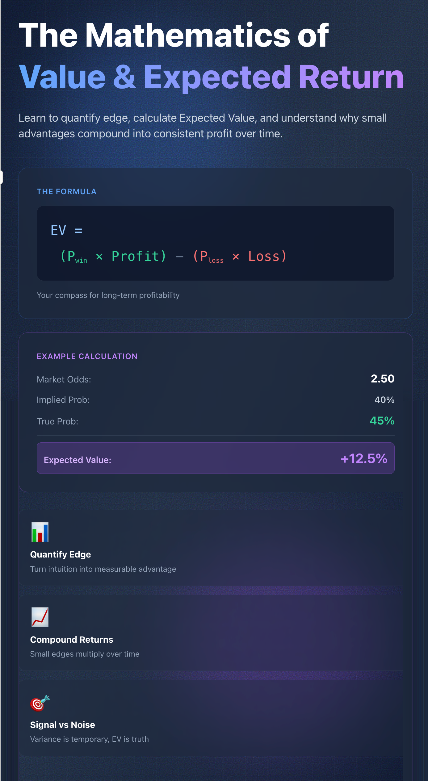
We’ll learn how to measure value, compare potential bets, and calculate expected value. This metric is what distinguishes professionals from casual punters, though the distinction isn’t always obvious at first.
If Lesson 1 was mindset, Lesson 2 is the math that powers it.
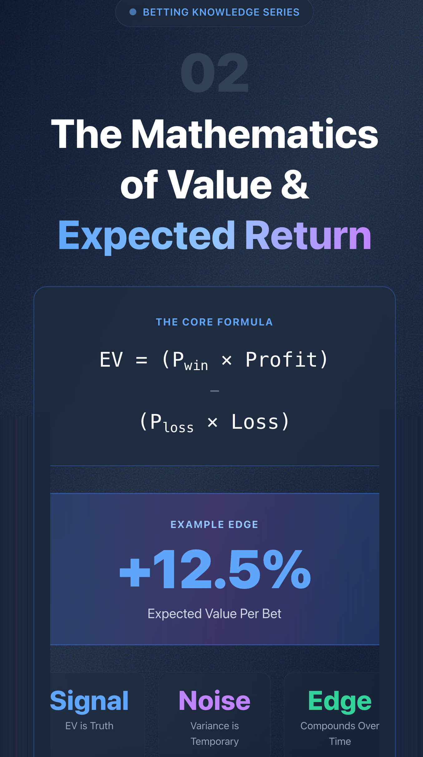
1. What Is Expected Value (EV)?
Expected Value (usually written as EV) is a way to quantify what you should win or lose per bet if you placed that same bet thousands of times.
It’s not a prediction of what will happen today. It’s the average result over time.
EV = (P_win × Profit_win) - (P_loss × Loss_loss)
In simple terms:
Multiply what you expect to win by the chance of winning, then subtract what you expect to lose multiplied by the chance of losing.
The result tells you whether that bet is profitable in the long run. Sometimes it feels counterintuitive when you’re staring at a single bet, but the math doesn’t lie.
2. Turning Odds Into Probability
Before you can calculate EV, you need to translate decimal odds into implied probability:
Implied Probability = 1 / Decimal Odds
Example:
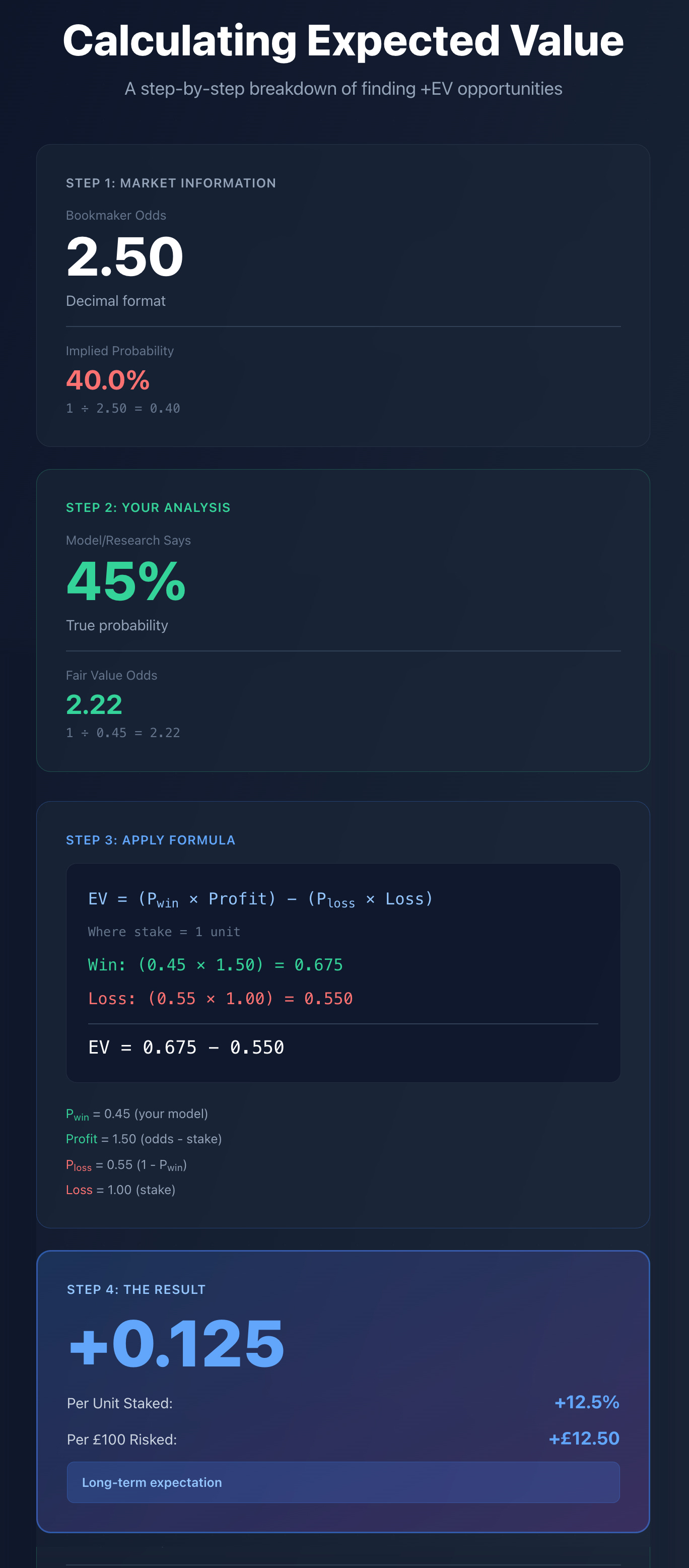
Odds = 2.50 → Implied Probability = 1 / 2.5 = 40%.
If your research or model says the true probability is 45%, then the market is underpricing that outcome.
That 5% gap is your edge.
3. Calculating EV in Practice
Let’s apply it.
You’re offered odds = 2.50 on an event.
Your model says it should be 2.22 (which equals 45% chance).
Step 1: Find the true vs. market probabilities
Market = 40%, True = 45%
Step 2: Plug into the EV formula
Profit if win = +1.50 (since 2.5 - 1 = 1.5 units gained per 1 staked)
Loss if lose = -1.00
EV = (0.45 × 1.5) - (0.55 × 1)
EV = 0.675 - 0.55 = +0.125
Your Expected Value = +0.125, or +12.5% per bet.
That means that in the long run, every £100 risked would yield an average profit of £12.50. Pretty straightforward once you see the numbers work.
4. Positive vs. Negative EV
EV Type Description Long-Term Outcome Positive (+EV) True Probability > Implied Probability Profitable over time Negative (-EV) True Probability < Implied Probability Losing over time
Most bettors live permanently in -EV territory because they bet for entertainment or intuition.
Professionals live in +EV territory, even if that means long streaks of variance. And the variance can be brutal.
5. Variance: Why +EV Doesn’t Mean Every Bet Wins
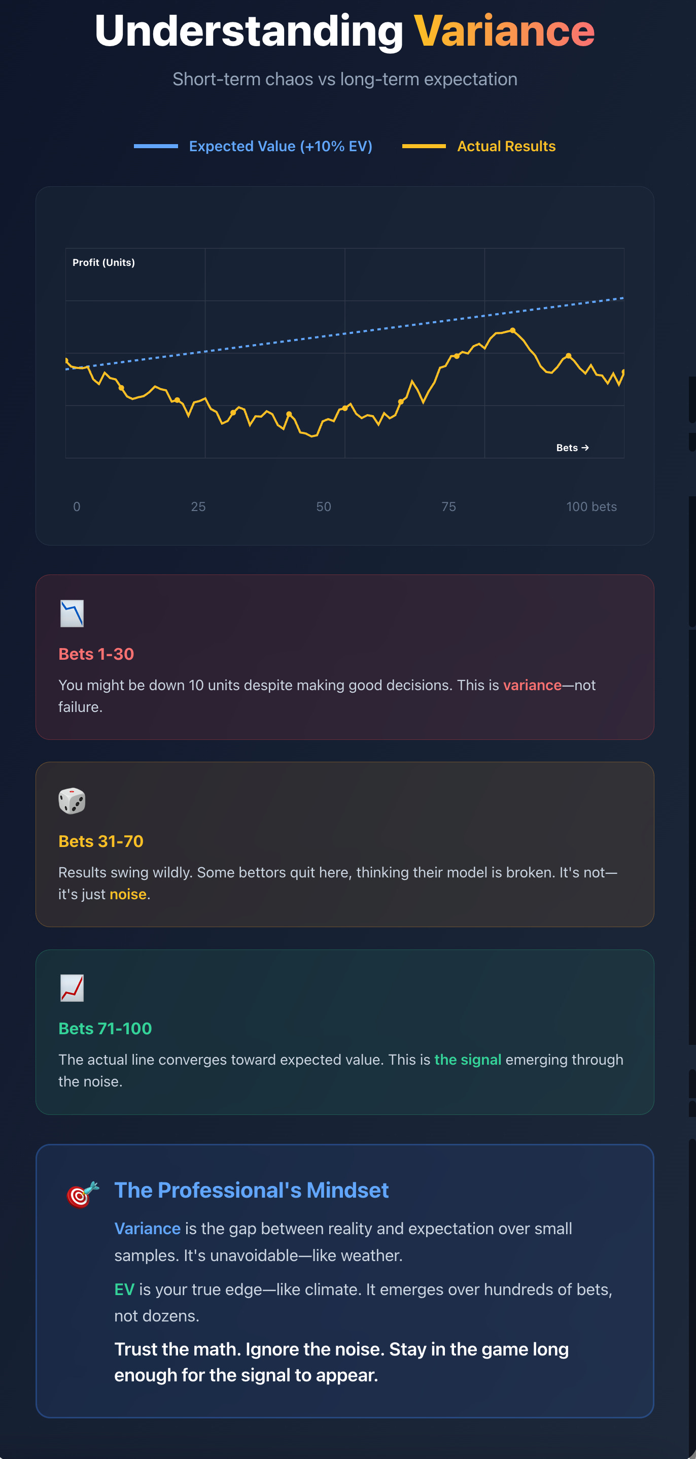
Even with a positive EV, short-term results can look chaotic.
That’s called variance. The natural fluctuation between expectation and reality.
Example:
You take 100 bets with +10% EV.
Mathematically, you should earn about 10 units profit. In reality, you might win 20 or lose 10 before the curve normalises.
Variance is the noise. EV is the signal.
Trust the signal, though I know it’s harder when you’re down 15 units.
6. Understanding Edge Size
Not every +EV opportunity is equal.
Small edges add up faster than you think, and big edges are rare.
Edge Description Typical Use +1-2% Marginal but repeatable Daily grind bets +5% Solid, reliable edge Core trading setups +10%+ Rare, strong mispricing Value bursts or special events
Professionals build portfolios of small edges. Hundreds of micro advantages compounding into consistent profit.
7. The Relationship Between EV and Bankroll Growth
Your bankroll’s growth rate depends on two things:
The size of your edge (EV).
The fraction of bankroll you risk (stake).
Stake too little → growth is slow.
Stake too much → volatility kills you.
Later in the Best Staking Plans series, you’ll learn how to match stake size to edge (like the Kelly Criterion), but the principle is simple:
The stronger your edge, the more you can responsibly stake, but never so much that variance can destroy you.
8. Applying EV Thinking in Real Markets
EV isn’t limited to match-odds markets.
It applies to every pricing environment. Goals, corners, cards, player props, even trading positions.
Example workflow for an xG-based trader:
Your model projects 2.90 total xG for a match.
Market’s Over 2.5 Goals odds = 1.95 (51% implied).
Your simulation suggests 57% chance → +6% edge.
That’s +EV. Execute the trade.
When you start viewing every market this way, the noise disappears. It’s just numbers and discipline.
9. Building a +EV Habit
Consistency beats brilliance. I’ve seen this play out more times than I can count.
Develop the habit of asking three questions before any bet:
What’s the true probability?
What’s the market’s implied probability?
Is there a gap big enough to justify risk?
If you can’t answer those three, you’re gambling, not trading.
10. Measuring Your Real-World EV
Keep a record of every bet: odds taken, model probability, result.
Over time you can calculate your realised EV:
Realised EV = (Total Profit / Total Staked) × 100
This tells you whether your theoretical edge is converting in reality.
If your realised EV trends positive over hundreds of bets, your model works. If it trends negative, refine your assumptions, not your luck.
Key Takeaways
✅ EV quantifies edge. It’s your compass for long-term profit.
✅ Positive EV doesn’t guarantee short-term wins, but it guarantees long-term growth.
✅ Small edges compound when executed with discipline.
✅ Variance is noise. Trust the math, not emotion.
✅ Always record and review your EV to validate your system.
Next Lesson
📘 Lesson 3: The Myth of “Safe Bets” and Why Probability Never Sleeps
We’ll explore why “guaranteed” bets don’t exist, how risk is built into every market, and how to think in probabilistic ranges rather than certainties. A mindset shift that distinguishes genuine traders from hopeful punters.